


👋 Hi, this is P.Y., I work as an Android Distinguished Engineer at Block. As we started evaluating the performance impact of software changes, I brushed up on my statistics classes, talked to industry peers, read several papers, wrote an internal doc to help us interpret benchmark results correctly and turned it into this article.
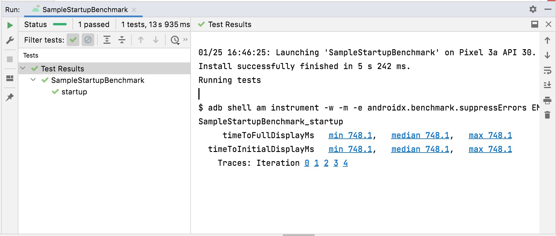
At Square, we leverage Jetpack Macrobenchmark to benchmark the UI latency of critical user interactions. We trace user interactions with Trace.beginAsyncSection and capture their durations with TraceSectionMetric.
The official documentation shows how to see and collect the results, but does not provide any guidance on interpreting these results in the context of a software change. That's unfortunate: the primary goal of benchmarks is typically to compare two situations and draw conclusions.
Should I compare the min, the median, or the max? If I get a difference of 1 ms, is that an improvement? What if I run the same 2 benchmarks again and get different results? How do I know I can trust my benchmark results?
The Statistically rigorous java performance evaluation paper demonstrates how comparing two aggregate values (e.g. min, max, mean, median) from a benchmark can be misleading and lead to incorrect conclusions.
This article leverages statistics fundamentals to suggest a scientifically sound approach to analyzing Jetpack Macrobenchmark results. If you're planning on setting up infrastructure to measure the impact of changes on performance, you should probably follow a similar approach. This is a lot of work, so you might be better off buying a solution from a vendor. I talked extensively with Ryan Brooks from Emerge Tools and was pleased to learn that they follow a similar approach to what I'm describing in this article.
Towards the end, I'll also provide an interpretation of the statistics behind the Fighting regressions with Benchmarks in CI article that the Jetpack documentation recommends as a resource.
I wasn't particularly strong at statistics in college. If you notice a mistake please let me know!
Deterministic benchmarks
In an ideal world, running a benchmark in identical conditions (e.g. a specific version of our software on specific hardware with a specific account) would always result in the same performance and the same benchmark results. Changing some of these conditions, e.g. the hardware or software, would provide a different result.
For example, let's say we have an ideal work benchmark where we run 100 iterations, and for each iteration the measured duration is always 242 ms. So the mean is 242 ms. We optimize the code, run the 100 iterations again, and the measured duration is now 212 ms for each iteration. We can conclude that we improved performance by 30 ms or 12.4%. But if every iteration yields a slightly different result, we can't make that claim.
💡 Deterministic measurements can be summarized with a mean or sum. Unfortunately, Jetpack Macrobenchmark runs are not deterministic. It's possible to design alternate benchmarking methods that don't rely on time but instead track deterministic measurements (e.g. number of CPU instructions, number of IO reads, number of allocations), which provide clear-cut results. However, when evaluating performance as perceived by humans, time is the only measurement that matters.
Fixed environment
If we change more than one condition at a time in between two benchmark runs (e.g. both the software and hardware), we can't tell if a benchmark result change is caused by a software change or hardware change.
So, as a rule of thumb, we should only have one changing variable between two benchmark changes. Since we're interested in tracking the impact of code changes (i.e. the app software stack), we need everything else to be constant (hardware, OS version, account, etc). For example, we should not compare one benchmark on a phone with version 6 of the app with another one on a tablet with version 7 of the app.
It's still worth running a specific benchmark with several varying conditions (phone, tablet, types of users, etc), as long as we only do paired comparisons of the before & after change.
Nondeterminism & probability distribution
With Jetpack Macrobenchmark, even though we're in a fixed environment (identical device, OS version, etc), we're still benchmarking incredibly complex systems with many variables at play, such as dynamic CPU frequencies, RAM bandwidth, GPU frequency, OS processes running concurrently, etc. This introduces variation in the measured performance, so every iteration will give us a different result.
💡 One core idea is that the performance our benchmark is trying to measure follows a probability distribution: a mathematical function that gives the probabilities of occurrence of different possible outcomes for an experiment (wiki). We don't know the actual function for that probability distribution.
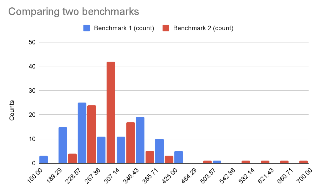
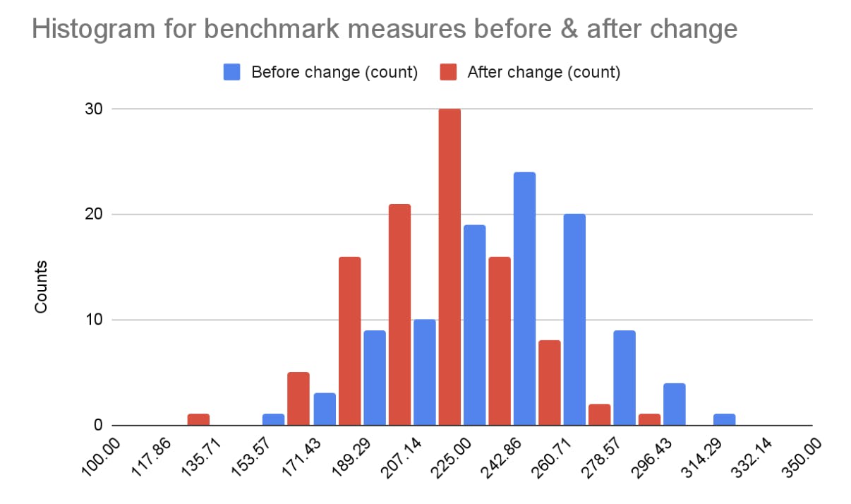
By running benchmarks before & after a change, we sample two probability distributions. We can draw histograms to get an approximate representation of the sample distributions. Let's look at an example:

The blue benchmark has a median of 295.8 ms and the red benchmark has a median of 292.9 ms. We could conclude that there's a 2.9 ms improvement, but the histograms show that these two sample distributions look very different. Is the red benchmark better than the blue one?
More importantly, if we run the before or the after benchmark several times, we will get a different median. Here, the difference in the medians is small enough that we might sometimes get better a median before the code change (blue), even though this time red was better.
We have to use statistical techniques to derive valid conclusions or surface inconclusive benchmarks.
Identifying sources of variation
In the previous chart, the first benchmark (blue) seems to have two modes (peaks). Instead of a histogram, we can graph the measured values in iteration order:
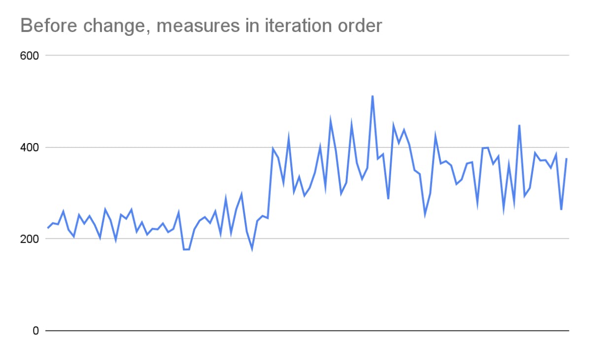
This tells a much different story! After investigating, we discover that this benchmark triggered thermal throttling: when a device temperature goes over a target, the CPU frequencies are scaled down until the temperature goes down. As a result, everything on the device runs slower.

We can work around this variance by avoiding thermal throttling: using a device with better thermal dissipation, running the benchmark in a colder room, or running the entire benchmark at a lower CPU frequency.
Similarly, notice how the red histogram above has a long right tail with a few high measures. Graphing the benchmark in iteration order, we see the following:
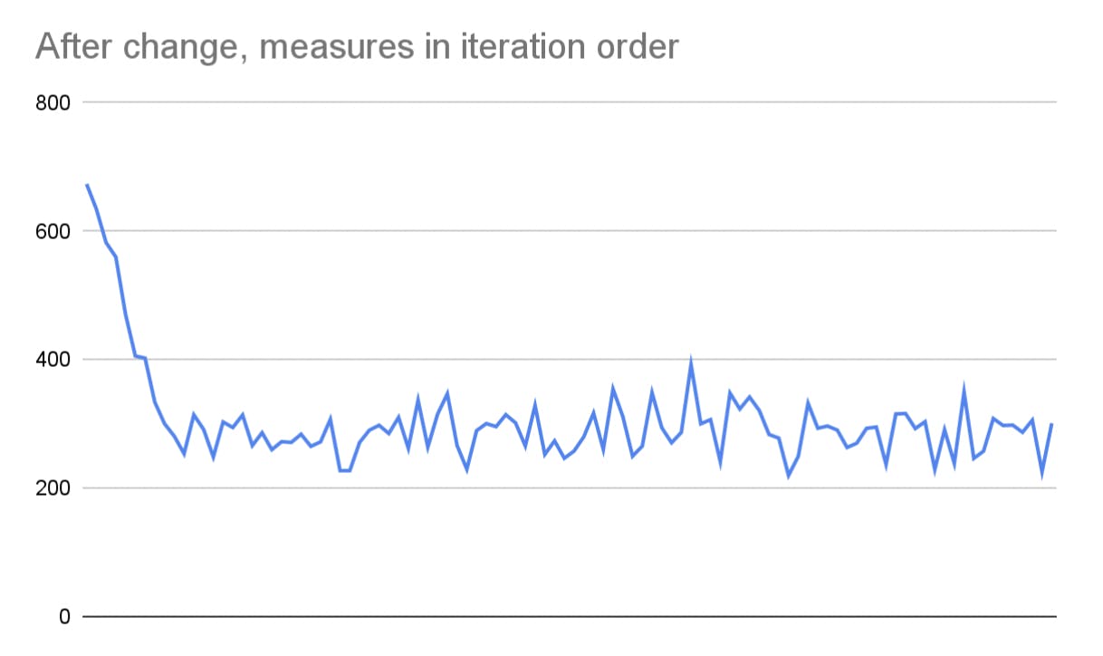
This looks like a warm-up effect, where the first iterations are slower, due to e.g. cold caches or JIT compilation. To work around this, we could install the app with full AOT compiling and perform warm-up iterations.
🤨 Should we leave these sources of variation in to keep the benchmarks realistic?
No. We evaluate the impact of the change as precisely as we can by removing as many variables as we can. If we want to measure performance with & without thermal throttling, or cold start performance, we can also test for those as separate benchmarks (e.g. keep the code identical and run the benchmark with and without thermal throttling to evaluate the impact that thermal throttling has on runtime performance).
Normal distribution
As we remove all identified sources of variation, the benchmark histograms start to look more and more like a bell curve, a graph depicting the normal distribution:
A normal distribution is a parametric distribution, i.e. a distribution that is based on a mathematical function whose shape and range are determined by distribution parameters. A normal distribution is symmetric and centered around its mean (which is therefore equal to its median), and the spread of its tails is defined by a second parameter, its standard deviation.
Comparing two normal distributions with a roughly equal standard deviation is easy: one distribution is simply shifted. Since they're symmetric around their mean we can just compute the difference between the two means.
However, we're not certain that the underlying distributions are normal, we can only estimate the likelihood that they're normal based on the sample data we got from the benchmark.
Normality fitness test
There are many popular normality tests to assess the probability that a set of sample measures follows a normal distribution. Unfortunately, the golden standard to this day seems to be the eyeball test, i.e. generate a histogram or a Q-Q plot and see if it looks normal. The eyeball test is hard to automate 😏.
The Comparisons of various types of normality tests study concludes that selecting the best fitness tests depends on the distribution shape:
For symmetric short-tailed distributions, D’Agostino and Shapiro–Wilk tests have better power. For symmetric long-tailed distributions, the power of Jarque–Bera and D’Agostino tests is quite comparable with the Shapiro–Wilk test. As for asymmetric distributions, the Shapiro–Wilk test is the most powerful test followed by the Anderson–Darling test.
The DatumBox Framework provides a ShapiroWilk.test() function that we can use to assess if the measures are not normally distributed, in which case we shouldn't use the benchmark results as is and need to perform additional work to fix error sources.
// alpha level (5%): probability of wrongly rejecting the hypothesis that the distribution is normal (null hypothesis).
val alphaLevel = 0.05
val rejectNullHypothesis = ShapiroWilk.test(FlatDataCollection(distribution), alphaLevel)
if (rejectNullHypothesis) {
  error("Distribution failed normality test")
}
Sample mean difference

In the example above, the data for the first benchmark was generated by sampling two normal distributions, one with a mean of 242 ms and the other with a mean of 212 ms, so the real mean difference was 30 ms. However, the first sample distribution has a mean of 244 ms and the second has a mean of 209 ms, so the sample mean difference is 35 ms, 17% higher.
As you can see, even if the likelihood of normality is high enough, we don't know the actual real means of the underlying distributions, so we can't compute the exact difference between the two real means, and the difference between the two sample means can be significantly off. However, we can compute a likely interval for where the mean difference falls.
Confidence interval for a difference between two means
It's formula time (source)! If the following is true:
Both benchmarks yield sample data that follows a normal distribution.
Each benchmark has more than 30 iterations.
The variance of one benchmark is no more than double the variance of the other benchmark.
Then the confidence interval for the difference of means between the two benchmarks can be computed as:
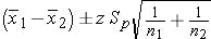
The confidence interval is the difference between the means, plus minus the margin of error.
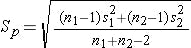
zis the Z score.Spis the pooled estimate of the common standard deviation, computed as:
Note: if the confidence interval crosses 0 (i.e. the interval goes from a positive value to a negative value) then the benchmarks do not demonstrate any impact for the change.
In this example above, the real mean difference from normal distributions used to generate sample data was 30 ms. The sample mean difference was 35 ms, but if we sample again we'll get another mean difference. The formula shared above allows us to say that the 95% confidence interval of the mean difference is an improvement of somewhere between 24.92 ms and 45.10 ms. If we run the two benchmarks 100 times, there's a 95% probability that the sample mean difference will fall in that interval.
In other words, we're fairly confident that the real mean difference is somewhere between 24.92 ms and 45.10 ms. But we can't get any more precise than that unless we remove the sources of noise or increase the number of iterations by the square of the target increase. E.g. if we wanted to divide the confidence interval range by 3, we'd need to multiply the number of iterations by 9, from 100 to 900 iterations 🤯.
Coefficient of variation check
The confidence interval grows linearly with the standard deviation, so if we want our benchmarks to be conclusive we need to keep the standard deviation in check. One way to do this is to compute the Coefficient of Variation (standard deviation divided by mean) for each benchmark and ensure that it's below a threshold.
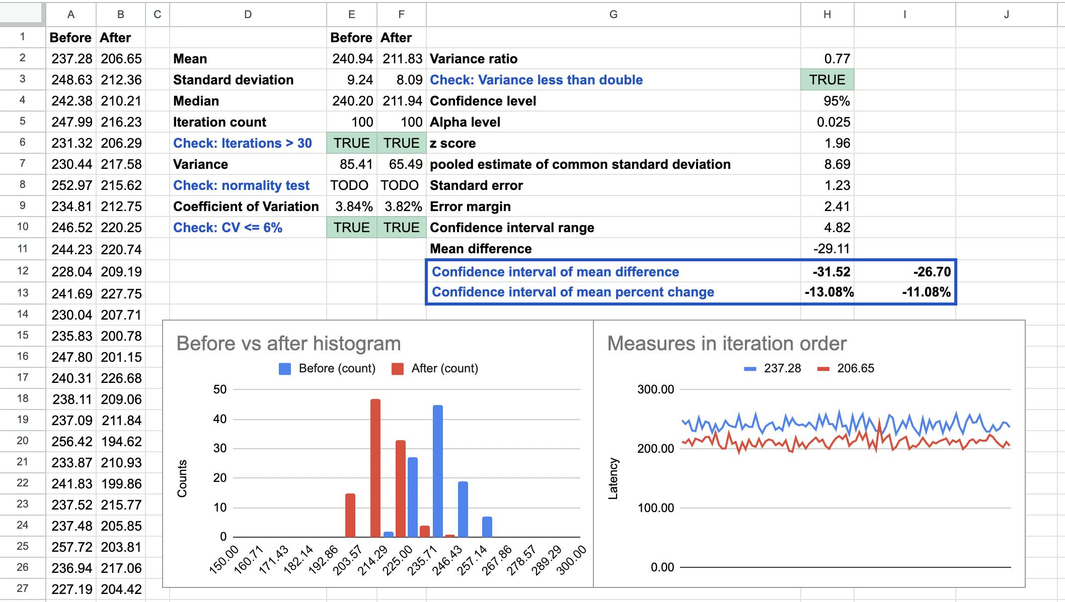
Putting it all together
I created a Google Spreadsheet template that does most of the stats math for you (except the Shapiro-Wilk normality test) so that you can easily compute the impact of a change and the validity of your benchmarks. Click USE TEMPLATE and paste the iteration results of each benchmark runs.
What if the benchmarks aren't normally distributed?
Remove sources of variation
You can fix a benchmark distribution that doesn't look normal by fixing sources of variation. The simplest way to do this is to open the perfetto trace for the slowest iteration and the faster interaction, figure out what's causing the difference and fix it.
Remove outliers
If we cannot isolate & remove error sources, we can try to eliminate them by cleaning up our data set, in 2 ways:
Implement a sliding window such as only the last N iterations of a run are considered. This helps with sources of variation like classloading or JIT compiling. This is effectively the same as performing a benchmark warm-up.
Eliminating outliers
Tukey's fences: removing values that are below Q1 - 1.5 IQR or above Q3 + 1.5 IQR. Note: Q1 = p25, Q3 = p75, IQR = Q3 - Q1.
Another approach is to discard outliers that are more than ~2 standard deviations from the mean.
This can work if the distribution does otherwise have a normal shape.
Generally speaking, you're better off investigating and finding the root cause rather than blindly removing outliers.
Try a log-normal distribution fit
From Scientific Benchmarking of Parallel Computing Systems:
Many nondeterministic measurements that are always positive are skewed to the right and have a long tail following a so-called log-normal distribution. Such measurements can be normalized by transforming each observation logarithmically. Such distributions are typically summarized with the log-average, which is identical to the geometric mean.
I haven't spent too much time looking into this as our distributions pass normality tests.
Kolmogorov–Smirnov test
From Wikipedia:
The Kolmogorov–Smirnov test is a nonparametric test of the equality of continuous, one-dimensional probability distributions that can be used to compare a sample with a reference probability distribution (one-sample K–S test), or to compare two samples (two-sample K–S test).
We can leverage this test to compute the probability that our two benchmarks are from the same probability distribution, to establish whether a change has a statistically significant impact on performance. However, this won't tell us anything about the size of that impact.
Central Limit Theorem
From Wikipedia:
The central limit theorem (CLT) establishes that, in many situations, for identically distributed independent samples, the standardized sample mean tends towards the standard normal distribution even if the original variables themselves are not normally distributed.
When we run a benchmark several times and keep the mean for each run, that mean will be normally distributed around the real mean of the underlying benchmark distribution. If we do this before and after the change, we now have 2 normal distributions of means.
We can leverage this to detect regressions by applying a two-sample t-test which will tell us the probability that the two normal distributions of means have the same mean. If they don't, then we can conclude that the underlying benchmark distributions have a different mean, i.e. that there is a change, but we can't conclude much in terms of the impact of the change.
This approach is what Google has been recommending in an article frequently referenced by Android developers: Fighting regressions with Benchmarks in CI. The article calls it "step-fitting of results" and doesn't mention the CLT or two-sample t-tests, probably because the technique was copied over from Skia Perf.
If you assume that sources of variation are a fact of life and that you won't be able to fix them and consistently get normal distributions with stable variance, then this approach is probably your best option.
Running N benchmarks before and after a change is a lot more expensive, so the suggested approach is to run a single benchmark per change, wait until N/2 changes have landed, then separate the N benchmarks around the change in a before and after group. Alternatively, you could leverage bootstrapping.
Conclusion
Jetpack Macrobenchmark runs are non-deterministic. Don't look at aggregate values such as min, max, mean or median.
Check that the benchmark measures follow a normal distribution.
If not, find the root cause. Common fixes:
Killing / uninstalling unrelated apps.
Setting the device to Airplane Mode during the measured portion.
Full AOT compiling of the APK.
Locking CPU frequencies.
Stable room temperature.
Plugging in the device to power.
Killing Android Studio and anything that might run random ADB commands while profiling.
Compute the confidence interval for a difference between two means (see this Google Spreadsheet template), that's the result you want to share. Remember to share just the interval and hide the specific sample mean difference from the 2 benchmarks you ran, as it has no meaning.